Can find live-written Mathematica notebook for all 4 lectures here.
Video for [Lecture 1] [Lecture 2] [Lecture 3] [Lecture 4]
Link to all summer school lectures, hosted by the Higgs Center for Theoretical Physics in Edinburgh, here.
Other lecturers: Stefan Weinzierl, Marcus Spradlin, Jaroslav Trnka, and Johannes Henn.
Also nice research presentations by: Jorrit Bosma, Sebastian Mizera, Gustav Mogull, Chia-Hsien Shen, Andrew McLeod, Theresa Abl, Joe Farrow, and Andres Luna-Godoy.
Lectures
Introducing graph methods for modern amplitude calculation. Topics:
-
Graphs and Ordered Amplitudes
-
Integrand Verification – two-loops.
-
Integrand Cut Construction – two loops.
-
Introduction to Color-Kinematics
Unsatisfactory tensile strength of one leg, combined with a fairly local interaction of a skateboard and an ill-chosen hill on a novel commute route, necessitated a little creativity in lecturing – black boards are out for at least another month. I didn’t want to present a straight-up slide show which I find a little off-putting for lectures. Rather I decided to (for the first time as a lecturer) live-generate a Mathematica notebook as the projected lectures. Obviously this could be incredibly off-putting, but this I indulged, as it’s the type of thing I would’ve loved to see when I entered this field in 2006.
Indeed, I organized around what I had to do as a early-stage graduate student to think through and understand the graphical mechanics behind the first paper that made sense to me re: the unitarity method – the groundbreaking 1998 two loop maximally supersymmetric supergravity calculation of Bern, Dixon, Dunbar, Perelstein and Rozowsky. You can find the paper here.
I start by introducing the need for graphs with structure to encode the types of minus signs that show up around vertex flips for adjoint color-weights. I explain how to generate the graphs contributing to unitarity cuts and how to dress them with a candidate graphically organized integrand (mapping from graphs to weights). We poke at what’s necessary to constrain a graphically organized integrand to match a given theory, and at the end delve into constraints that have nothing to do with physical observation but have everything to do with lining up local stories relating gauge theory and gravity predictions.
I did a little post-cleanup to make it somewhat more readable for people who don’t get to hear my vocalizations, but have posted sooner rather than indulge ever-present obsessive impulses towards stand-alone readability.
I don’t emphasize it but I’ve dropped in some pretty chonto casually tossed off calculations like automatically taking gauge integrands to symmetric double-copy gravity cuts via KLT, and evaluating 4D state sums for generic cuts in choose-your-SUSY gauge theories at the push of a button. As these weren’t (primarily) graphical methods they weren’t central to these lectures, but I can probably be tempted into writing some words about them at some point.
Notebook uses my github hosted amplitudes graph library ampGraphTools. (No need to install the library, it imports directly from github if the lectures’ notebook is executed.) Presented with an emphasis on output, not so much on code/library use, but does provide a slice of insight into how I actively think through this graphical playground when I’m poking about.
As a side note, I saved the notebook periodically throughout my lecture, and had it temporarily hosted on a dropbox folder accessed via a bit.ly link for students to grab as they liked. Interesting to see the stats of how many students bothered to grab the notebook vs who couldn’t care less.
Definitely welcome any questions, desire for clarification, and requests for any topics I skipped in this limited lecture time.


